Lesson summary “Editing a spreadsheet”
Lesson Topic: Editing a Spreadsheet
Lesson objectives:
- Educational: teach students to perform the following operations:
– selection of cell ranges;
– clearing cells and ranges;
– copying and moving the contents of cells and ranges;
– inserting and deleting cells, rows, columns.
- Developmental: learn to build analogies, highlight the main thing, pose and solve problems.
- Educational: to cultivate accuracy, attentiveness, politeness and discipline.
Lesson type: learning new material.
Equipment: software, textbook.
During the classes:
- Organizational moment (1 min);
- Updating knowledge (3 min);
- Learning new material (13 min);
- Homework (1 min);
- Practical part (25 min);
- Summing up the lesson (2 min).
During the classes
1. Organizational moment.
Checking students' readiness for the lesson.
2. Updating knowledge.
1. What is a spreadsheet ? (a set of data stored in computer memory that is displayed in the form of a table);
2. What are table processors ? (application program designed to work with spreadsheets);
3. Which table processor are you already familiar with? (Microsoft Excel);
4. What is a cell range ? (a collection of several cells).
3. Studying new material.
You already know how to select individual cells and edit the data they contain. Today in the lesson we will learn how to work with ranges of cells and consider the following operations:
– selection of cell ranges;
– clearing cells and ranges;
– copying and moving the contents of cells and ranges;
– inserting and deleting cells, rows, columns.
Selecting cell ranges
Selecting a cell makes it active and its name (address) appears in the names field.
Recall that a special notation is used to designate ranges of cells: for example, A1:E1 corresponds to a row of five cells, and E5:E8 corresponds to a column of four cells.
You can select a range of cells using the mouse or keyboard.
To select a range of cells, first select one of its outermost corner cells. To do this, place the mouse pointer on it and click the left button. While holding the button down, drag the pointer over the remaining cells in the range and release the button.
Non-contiguous (i.e. not touching) ranges are highlighted with the Ctrl . It is released after the selection of all ranges is completed.
To select a range of cells using the keyboard, you must move to the outermost cell of the range using the cursor keys. Then, while holding down the Shift , use the movement keys to select the remaining cells and release Shift .
Cleaning cells
To delete the contents of cells and ranges, simply select them and press the Del . On the Home , clicking the Clear opens a submenu with commands that allow you to delete only the contents of cells, formats, notes, hyperlinks, or all at once.
Copying and moving cell contents
To copy (move) data from one place on a sheet to another, you can use the Copy (Cut)→Paste on the Home or the key combination Ctrl+C (Ctrl+X)→Ctrl+V . When you run the Copy (Cut) , the selected range of cells is surrounded by a dotted line, and its contents (including notes and formatting) are placed on the clipboard. When you run the Paste , this content from the clipboard is placed in a new location, replacing the content that is there. You can stop performing operations by pressing the Esc .
Note that the Cut does not apply to moving non-adjacent ranges of cells. Also, unlike other Windows applications, after cutting, the contents of the buffer can only be pasted once. To perform multiple insertions, use the Copy (or the key combination Ctrl+C ).
The fastest and most visual way to move a range of cells is to drag (drag) the mouse from one place on the sheet to another. To perform this operation, you first need to select the desired range of cells (usually using the mouse). Then release the left mouse button and move the cell pointer (white cross) to the selection border so that it looks like a black cross with an arrow at the bottom. Next, you need to press the left mouse button and drag the selected cells to the desired location. To make it easier to select a location while moving, the selected range, the outline of the one being dragged, and its new address are displayed.
Ctrl key while dragging .
Inserting and deleting rows, columns, and cells
New rows and columns are added to a worksheet as follows: on the Home Insert button , you can open a submenu with the commands Insert Rows into Worksheet and Insert Columns into Worksheet .
Inserting a new row moves existing rows down. Inserting a column shifts existing columns to the right. When adding a line, select the line before which you want to insert a new line. A line is highlighted by clicking on its number. When adding a new column, select the column to the left of which you want to insert a new column. A column is highlighted by clicking on its letter designation.
Inserting individual cells into rows or columns of a sheet is performed using the commands Insert→Insert Cells . In this case, in the dialog box that appears, they indicate where the cells should be shifted when inserting - down or to the right.
Deleting cells, rows or columns is performed as follows: by clicking the Delete on the Home , a submenu with the commands Delete cells , Delete rows from sheet , Delete columns from sheet is called up .
When you select the Delete Cells , in the dialog box that appears, you select what you want to delete and where to move the cells when deleting.
Cancel and revert changes
At any time, the user has the opportunity to cancel the last changes made. , you can use the Cancel , which is located in the upper left corner above the ribbons, or the key combination Ctrl + Z. Revert button , or the key combination Ctri+Y , allows you to return a canceled command.
Example 1: Perform the required operations on cell ranges.
Let's select the range B5:B11 (7 cells from B5 to B11 ). To do this, place the mouse pointer in the form of a cross on cell B5 , press the left mouse button and, without releasing it, drag the selection (of a darker color) up to and including cell B11 .
Move the mouse pointer to one of the selection boundaries (the white cross will turn into a black cross with arrows) and, holding the left button, drag the selected data to column D.
In a similar way, drag the cells to their original location.
Dragging cells while holding down the Ctrl causes data to be copied. In this case, a plus sign appears to the right of the light arrow. Select 10 cells A6:B10 and copy their contents to the range C4:D8 .
Let us remind you that you can also copy and move data using the Paste , Cut or Copy on the Home , or by right-clicking and calling up the context menu, or by using the key combinations Ctrl+X (cut), Ctrl+C (copy), Ctrl+V (paste).
Select two columns A and B and copy their contents to Sheet2 , columns D and F (switch the sheet by clicking on the shortcut at the bottom of the window).
Select and clear all cells of Sheet2 (by selecting the command Clear→Clear all ). Let's go back to Sheet1 .
Selecting non-adjacent ranges of cells is carried out while pressing the Ctrl . Select the range of cells A4:B6 , press the Ctrl and, while holding it, select the range of cells A10:B11 . contents to the clipboard and paste them into columns D and E.
4. Homework.
§12, questions 1-3.
5. Practical part.
For completing this task you can receive a maximum of 7 points. To get 8-9 points you must answer questions. To get 10 points you need to complete an additional task.
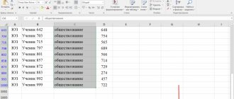
Task 1. Open the book upr12.xls. Some rows or columns in the tables are mixed up. Correct the table using copy, move, delete, and insert operations.
A)
b)
V)
G)
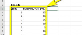
Task 2. Create a table and perform calculations.
- Calculate Profit ( =B3-B2 ) and Income Tax ( =B4*20% ).
- Using the SUM , calculate the Total .
- Use the AVERAGE to calculate the Quarterly Average .
- Column G is calculated using the formula: = D / C *100%
Result:
6. Summing up the lesson.
1. What actions can be performed with selected ranges?
2. How can you copy (move) the contents of cells?
3. How can I delete a row, column, or cells in a spreadsheet? Insert row, column, cells?
Grading.
Abstract on the topic “Spreadsheets”
Spreadsheet
is an application program for working with large arrays of numerical information. An electronic table (ET) allows you to store in tabular form not only a large amount of source data and calculation results, but also mathematical relationships between them, the values of which are automatically recalculated using specified formulas when the values of the source data change.
Main areas of application of ET
- calculation of the use of funds in financial transactions
- statistical data processing
- mathematical modeling of processes
- engineering calculations.
Basic Spreadsheet Functions
- calculations involving data in a table;
- searching and sorting information;
- graphic display of numerical information from a table (construction of graphs and diagrams);
- statistical data analysis.
Launch
Excel :
Start – All Programs – Microsoft Office – Microsoft Excel.
Microsoft Excel window structure
- header line
- menu bar
;
- toolbar
(contains buttons for the most frequently used commands);
- format bar
;
- name field
(indicates the name of the selected cell);
- formula bar
(used to enter and edit cell contents);
- Workspace;
- sheet tabs;
- scroll bars
.
A document in Microsoft Excel is called a workbook.
Workbook files have the extension . xls
or . xls x.
The workbook consists of sheets (three sheets are displayed by default when launched). The minimum element of an ET is called a cell.
Strings
in ET they are designated by numbers,
columns
– by letters of the Latin alphabet.
Cell address
indicated as follows:
- first indicate the column name (A, B, C, D, ….)
- then specify the name of the string.
For example:
A1, B2, C5, D11
Cell range
is a collection of several cells.
For example:
C4:C9 – elements of column C from 4th to 9th.
A3:D11 – rectangular range elements
Data input
– this is writing information into cells: text, numbers, formulas.
Data entry is carried out in two ways:
1. Using the formula bar:
To do this, you need to select the cell
,
click in the formula bar and enter the data. The following buttons will appear on the left:
X
( Esc )
– exits editing mode without saving changes;
V
( Enter )
– exits the editing mode and saves the changes.
2. Direct way:
select the cell and enter data (in this case, the data entered into the cell will be displayed in the formula bar).
Methods for editing data
- select a cell and enter new data (in this case, the previously entered cell contents will be lost);
- double-click on the cell and make the necessary changes;
- select the cell, press the key F2
and make the necessary changes;
- Select the cell, click in the formula bar and enter changes.
The list of formats is called up using the context menu command Format Cells.
Format Cells
dialog box, you need to open the
Number
and select the desired number data format. There are also Boolean values, True and False, used in comparison operations.
Examples of numeric data formats:
general, numeric, monetary, financial, text, percentage, fractional, date, time
, etc.
Using formulas in ET
Formulas in
Microsoft Excel are
expressions that describe calculations in cells.
Formulas fit into the formula bar.
Writing a formula begins with the “=” symbol.
Formulas may include the following components:
- the “=” symbol (the writing of the formula begins with it)
- operators, i.e. instructions for performing actions (+, -, *, /, etc.)
- data (numbers or text)
- functions
- cell and range references.
Examples:
= A1+B1;
= 0.2*D6;
= SUM(A3:A5).
Calculation of formulas
1.
write the “=” sign in the formula bar
2. enter the formula using the signs of arithmetic operations (+, -, *, /,%), numbers and cell names
Example.
=2.5*A1
= 3.75/С2
= A3+C4
Operators
in Microsoft Excel _
- text operator (
& - concatenation ) - address operators ( used to specify cell references )
- arithmetic operators
| Operator symbol | Operator name | Example formula | Result |
| + | Addition | =1,5+2,6 | 4,1 |
| — | Subtraction | = 4,8-3,2 | 1,6 |
| * | Multiplication | = 0,5*8 | 4 |
| / | Division | = 6/5 | 1,2 |
| % | Percent | = 40% | 0,4 |
| Exponentiation | = 3^2 | 9 |
4. comparison operators
| Operator symbol | Operator name | Example formula | Result |
| More | = 57 | Lie | |
| Less | = 4 | True | |
| = | Equals | = 5=9 | Lie |
| Less or equal | = 3 | Lie | |
| = | More or equal | = 4=4 | True |
| Not equal | = 56 | True |
Operator precedence
- Address operators.
- Negation operator.
- Percent.
- Exponentiation.
- Multiplication and division.
- Addition and subtraction.
- Text operator.
- Comparison operators.
Using built-in functions in a spreadsheet environment
Functions
are instructions that calculate a result by processing arguments.
Function arguments are written after its name in parentheses separated by semicolons.
To call the Function Wizard, you must execute the command Insert – Function
or click on the
f ( x )
in the toolbar.
Some standard features
| Name | Designation | Description of action |
| Math- tic | SIN(x) | calculating the sine of an angle |
| COS(x) | calculating the cosine of an angle | |
| ABS (x) | calculating the modulus of a number | |
| DEGREE (number; degree) | calculates the power of a given number | |
| SUM (argument list) | calculating the sum of argument values | |
| ROOT (number) | calculating the square root of a number | |
| Statistical tic | AVERAGE (argument list) | Calculation of the arithmetic mean of the arguments |
| MAX (argument list) | Calculating the maximum value among arguments | |
| MIN (list arguments) | Calculating the minimum value among arguments | |
| Logic function | IF (logical expression; expression 1; expression 2) | If the logical expression is true, then the function takes the value of expression 1, otherwise - the value of expression 2 |
Examples
| Example formula | Result |
| = SUM(2, 4.5) | 6,5 |
| = DEGREE (2, 5) | 32 |
| = SQRT(64) | 8 |
| =MAX (8,12,24,16) | 24 |
| =MIN (2,5,11,7) | 2 |
| = AVERAGE(6,8,10,12) | 9 |
SUMIF function:
SUMIF (range; criterion; sum range) – sums the cells specified by the specified condition
COUNTIF function:
COUNTIF (range; criterion) – counts the number of non-empty cells in the range that satisfy a given condition
Building charts and graphs
Charts and graphs, as you know, are designed to visually present data and make it easier to understand large amounts of data. Microsoft Excel also provides this capability. Diagrams are usually located on a worksheet and allow you to compare data and find patterns. Microsoft Excel provides extremely broad capabilities in creating all kinds of charts.
Types of charts in
Microsoft Excel :
pie, histogram, bar, graph, radar, donut, etc.
Creating Charts Using the Chart Wizard
- select areas of data on which the diagram will be built;
- call the Diagram Wizard (execute the command Insert – Diagram
or click on the corresponding button in the toolbar);
- select the chart type and click the Next button;
- change the data range (if necessary) and click the Next button;
- set the necessary chart parameters: title, axis labels, value labels and click the Next button;
- set the chart placement and click the Finish button
Changing individual chart options
- select the diagram (click on the diagram with the mouse);
- select menu item Diagram
(or call the context menu);
- Select the required command from the menu that appears;
- in the window that appears, set the necessary parameters;
- Click on the Ok button.
A quick way to create charts
- select areas of data on which the diagram will be built;
- press the F11 .
In this case, Microsoft Excel will build a standard type of chart on a separate sheet based on the selected range.
Printing charts
- highlight the diagram;
- execute command File - Print
(or press the key combination
Ctrl + P
); - set switch Selected chart
;
- Before printing, view the diagram (click the View button);
- set the number of copies;
- press the Ok button.